Hi! Great day! Welcome to this course. Thank you for taking an interest in this course. Learning from this course will help you become a Professional.

Lesson 1: Random variables, probability distributions

Course:

The subject of random variables plays an important part in any probability distributions. The term random variable is often associated with the idea that value is subject to variations due to chance. We often encounter random variables in library science literature with two specific outcomes:  discrete distribution and binomial distribution.

In R, to generate a random integer between 1 and 40 , we use the sample function:
>sample(1:40,4)
[1]  2 21  6  9

Another way to generate a random number is using the runif function.  This function will allow us to select a number between minimum and maximum that is equally likely to occur.
>x1 <- runif(1, 5.0, 7.5)
>x1
[1] 6.715697
In this function, it allows us to generate one random integer between 5.0 and 7.5.

A Discrete Distribution is a random variable  defined as a countable variable. To illustrate this type of distribution, let’s take the number of copies of Dostoyevsky’s Humiliated and Insulted found in the library. This number will not change as long as the library keeps track of these copies.

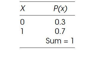
In order to illustrate discrete distributions, we will use the Bernoulli distribution. Bernoulli was known for his work on probability statistics and was one of the founders of the calculus of variations. Under this distribution there are only two possible values of the random variable, x = 0 or x = 1. When drawing numbers from this distribution, if selecting x = 0, the probability is P(x) = 0.3, while the probability of selecting x = 1 is 0.7.

However, we still need to find out the Mean and Standard Distribution in order to fully evaluate its values. The mean of a discrete variable is denoted by μ (mu). It is the actual mean of its probability. It is also called the expected value and is denoted by E(x). The mean or expected value of a discrete variable is the value that we expect to observe per repetition of the experiment we conduct over a large number of times.

To calculate the mean of a discrete random variable x, we multiply each value of x by the corresponding probability and sum (hence the symbol, Σ). This sum gives us the mean (or expected value) of the discrete random variable x. The formula for the expected discrete random variable is: μ = ΣxP(x)

In R, we use the table above for the two variables x and p. To calculate the mean, we need to multiply the corresponding values of x and p and add them.  We will call the result of this calculation mu.

>x <– c(0,1)
>p <–c(0.3, 0.7)
>mu <- sum(x * p)
>mu
[1] 0.7

The result 0.7 is the value of the mean.

The Standard Deviation of a discrete random variable is denoted by σ (sigma) and measures the spread of the probability distribution. A higher level for the standard deviation of a discrete random variable indicates that x can assume values over a larger range from the mean. In contrast, a smaller value for the standard deviation indicates that most of the values that x can assume are clustered closely to the mean. The formula for the standard deviation of a discrete random variable consists of:

In order to use R to calculate the value of σ square, we subtract the value of mu from each entry in x, square the answers, multiply by p, to reach the sum.

>sigma2 <- sum((x-mu)^2 * p)
>sigma
[1]  -2.17

The second form of discrete probability distribution is Binomial Distribution. It describes the behavior of a count variable x if the following conditions apply:
1: The number of observations n is fixed.
2: Each observation is independent.
3: Each observation represents one of two outcomes (“success” or “failure”).
4: The probability of “success” p is the same for each outcome

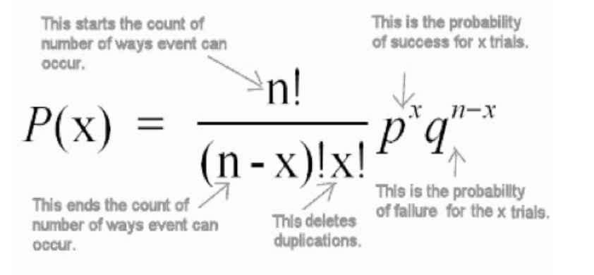
where P(x) = Probability of x success given the parameters n and p
n = sample size
p = probability of success
1 – p = probability of failure
x = number of successes in the sample (x = 0,1,2,3,4……n)

The binomial distribution in R is noted as dbinom. There are three required arguments for binomial calculation: the value(s) for which to compute the probability (k), the number of trials (n), and the success probability for each trial (θ). In the previous example, we employed all three values that include: 2 as the probability value of k,  2 is the number of trials , and 0.7 for success probability for each trial.

>dbinom(2, 2, 0.7)
where (x = 2, size = 2, prob = 0.7)
[1] 0.49

In R, the argument is pursued in the following manner:
x, q = vectors of quartiles
P = vector of probabilities
n = number of observations. If length (n) > 1,  the length is taken to be the number required.
size = number of trials

Lesson 2: Measures of central tendency and variability; higher-order moments

Course:

Central tendency

Definition: the tendency of quantitative data to cluster around some central value. The closeness with which the values surround the central value is commonly quantified using the standard deviation. They are classified as summary statistics

Measures of Central Tendency

1. Mean: The sum of all measurements divided by the number of observations.Can be used with discrete and continuous data. It is value that is most common
2. Median: The middle value that separates the higher half from the lower half. Mean and median can be compared with each other to determine if the population is of normal distribution or not. Numbers are arranged in either ascending or descending order. The middle number is than taken.
3. Mode: The most frequent value. It shows most popular option and is the highest bar in histogram.Example of use: to determine the most common blood group.
4. Geometric mean – the nth root of the product of the data values.
5. Harmonic mean – the reciprocal of the arithmetic mean of the reciprocals of the data values.
6. Weighted mean – an arithmetic mean that makes use of weighting to certain data elements.
7. Truncated mean – the arithmetic mean of data values that do not include the whole set of values, such as ignoring values after a certain number or discarding a fixed proportion of the highest and lower values.
8. Midrange – the arithmetic mean of the maximum and minimum values of a data set
9. ♙

Variability (dispersion)

Definition: dispersion is contrasted with location or central tendency, and together they are the most used properties of distributions. It is the variability or spread in a variable or a probability distribution Ie They tell us how much observations in a data set vary. They allow us to summarise our data set with a single value hence giving a more accurate picture of our data set.

Measures of variability

1. Variance: A measure of how far a set of numbers are spread out from each other. It describes how far the numbers lie from the mean (expected value). It is the square of standard deviation.
2. Standard deviation (SD): it is only used for data that are “normally distributed”. SD indicates how much a set of values is spread around the average. SD is determined by the variance (SD=the root of the variance).
3. Interquartile range (IQR): the interquartile range (IQR), is also known as the ‘midspread’ or ‘middle fifty’, is a measure of statistical dispersion, being equal to the difference between the third and first quartiles. IQR = Q3 − Q1. Unlike (total) range, the interquartile range is a more commonly used statistic, since it excludes the lower 25% and upper 25%, therefore reflecting more accurately valid values and excluding the outliers.
4. Range: it is the length of the smallest interval which contains all the data and is calculated by subtracting the smallest observation (sample minimum) from the greatest (sample maximum) and provides an indication of statistical dispersion. It bears the same units as the data used for calculating it. Because of its dependance on just two observations, it tends to be a poor and weak measure of dispersion, with the only exception being when the sample size is large.

Lesson 3: Other descriptive measures of distributions

Course:

When we conduct research with only two central variables, these variables become the theme of our research methodology. In order to analyze the correlation between two variables, we consult bivariate statistics to search out the embedded information. The term correlation is often associated with the terms association, relationship, and causation.

We will only look at the Pearson sample correlation coefficient and its properties.

Pearson sample correlation coefficient measures the strength of any linear relationship between two numerical variables. A Pearson sample correlation coefficient attempts to draw a line of best fit through the data points of two variables. The Pearson sample correlation coefficient, r, indicates how far away all these data points are to this line of best fit, i.e., how well the data points fit this new model/line of best fit. Its value can range from -1 for a perfect negative linear relationship to +1 for a perfect positive linear relationship. A value of 0 (zero) indicates no relationship between the two variables.

The Pearson sample correlation coefficient formula: 

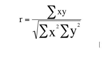
r = [Equation]
Σ = Number of pairs of sources
Σxy = Sum of the products of paired scores
Σx = Sum of x scores
Σy = Sum of y scores
Σx2 = Sum of squared x scores
Σy2 = Sum of squared y scores

In order to practice the Pearson sample correlation coefficient formula between two variables x and y, we will employ the data presented in the table below. In this table, the value x refers to the number of visitors to the special collections room in the library.  y stands for the number of visitors to the old newspaper archive collection room. Our objective is to compute the similarity between these two variables. The data for the two rooms used in our library research:

X	Y
Visitors to special collections room	Visitors to old newspaper archive collections room
1	4
3	6
5	10
5	12
6	13

Using Pearson sample correlation coefficient can show the correlation between the number of visitors to the special collections room and the number of visitors to both rooms. To achieve this value, Pearson sample correlation coefficient is computed by dividing the sum of the xy column (Σxy) by the square root of the product of the sum of the x2 column (Σx2) and the sum of the y2 column (Σy2).

Lesson 4: Joint distributions, conditional distributions, definitions of independence

Course:

Joint Distribution
3.1 Discrete case
Suppose X and Y are two discrete random variables and that X takes values {x1, x2, . . . , xn}
and Y takes values {y1, y2, . . . , ym}. The ordered pair (X, Y ) take values in the product
{(x1, y1),(x1, y2), . . .(xn, ym)}. The joint probability mass function (joint pmf) of X and Y
is the function p(xi
, yj ) giving the probability of the joint outcome X = xi
, Y = yj .
We organize this in a joint probability table as shown:
1
18.05 class 7, Joint Distributions, Independence, Spring 2014 2
X\Y y1 y2 . . . yj . . . ym
x1 p(x1, y1) p(x1, y2) · · · p(x1, yj ) · · · p(x1, ym)
x2 p(x2, y1) p(x2, y2) · · · p(x2, yj ) · · · p(x2, ym)
· · · · · · · · · · · · · · · · · · · · ·
· · · · · · · · · · · · · · · · · · · · ·
xi p(xi
, y1) p(xi
, y2) · · · p(xi
, yj ) · · · p(xi
, ym)
· · · · · · · · · · · · · · · · · ·
xn p(xn, y1) p(xn, y2) · · · p(xn, yj ) · · · p(xn, ym)
Example 1. Roll two dice. Let X be the value on the first die and let Y be the value on
the second die. Then both X and Y take values 1 to 6 and the joint pmf is p(i, j) = 1/36
for all i and j between 1 and 6. Here is the joint probability table:
X\Y 1 2 3 4 5 6
1 1/36 1/36 1/36 1/36 1/36 1/36
2 1/36 1/36 1/36 1/36 1/36 1/36
3 1/36 1/36 1/36 1/36 1/36 1/36
4 1/36 1/36 1/36 1/36 1/36 1/36
5 1/36 1/36 1/36 1/36 1/36 1/36
6 1/36 1/36 1/36 1/36 1/36 1/36
Example 2. Roll two dice. Let X be the value on the first die and let T be the total on
both dice. Here is the joint probability table:
X\T 2 3 4 5 6 7 8 9 10 11 12
1 1/36 1/36 1/36 1/36 1/36 1/36 0 0 0 0 0
2 0 1/36 1/36 1/36 1/36 1/36 1/36 0 0 0 0
3 0 0 1/36 1/36 1/36 1/36 1/36 1/36 0 0 0
4 0 0 0 1/36 1/36 1/36 1/36 1/36 1/36 0 0
5 0 0 0 0 1/36 1/36 1/36 1/36 1/36 1/36 0
6 0 0 0 0 0 1/36 1/36 1/36 1/36 1/36 1/36
A joint probability mass function must satisfy two properties:

1. 0 ≤ p(xi
   , yj ) ≤ 1
2. The total probability is 1. We can express this as a double sum:
   Xn m
   i=1
   Xp(xi
   , yj ) = 1
   j=1
   18.05 class 7, Joint Distributions, Independence, Spring 2014 3
   3.2 Continuous case
   The continuous case is essentially the same as the discrete case: we just replace discrete sets
   of values by continuous intervals, the joint probability mass function by a joint probability
   density function, and the sums by integrals.
   If X takes values in [a, b] and Y takes values in [c, d] then the pair (X, Y ) takes values in
   the product [a, b] × [c, d]. The joint probability density function (joint pdf) of X and Y
   is a function f(x, y) giving the probability density at (x, y). That is, the probability that
   (X, Y ) is in a small rectangle of width dx and height dy around (x, y) is f(x, y) dx dy.
   y
   d
   Prob. = f(x, y) dx dy
   dy
   dx
   c
   x
   a b
   A joint probability density function must satisfy two properties:
3. 0 ≤ f(x, y)
4. The total probability is 1. We now express this as a double integral:
   Z d
   Z b
   f(x, y) dx dy = 1
   c a
   Note: as with the pdf of a single random variable, the joint pdf f(x, y) can take values
   greater than 1; it is a probability density, not a probability.
   In 18.05 we won’t expect you to be experts at double integration. Here’s what we will
   expect.
   • You should understand double integrals conceptually as double sums.
   • You should be able to compute double integrals over rectangles.
   • For a non-rectangular region, when f(x, y) = c is constant, you should know that the
   double integral is the same as the c × (the area of the region).

Now we will introduce the concept of conditional probability.

The idea here is that the probabilities of certain events may be affected by whether or not other events have occurred.

The term “conditional” refers to the fact that we will have additional conditions, restrictions, or other information when we are asked to calculate this type of probability.

Let’s illustrate this idea with a simple example:

EXAMPLE:

All the students in a certain high school were surveyed, then classified according to gender and whether they had either of their ears pierced:

(Note that this is a two-way table of counts that was first introduced when we talked about the relationship between two categorical variables.

It is not surprising that we are using it again in this example, since we indeed have two categorical variables here:

• Gender:M or F (in our notation, “not M”)
• Pierced:Yes or No

Suppose a student is selected at random from the school.

• Let Mand not M denote the events of being male and female, respectively,
• and Eand not E denote the events of having ears pierced or not, respectively.

What is the probability that the student has either of their ears pierced?

Since a student is chosen at random from the group of 500 students, out of which 324 are pierced,

• P(E) = 324/500 = 0.648

What is the probability that the student is male?

Since a student is chosen at random from the group of 500 students, out of which 180 are male,

• P(M) = 180/500 = 0.36.

What is the probability that the student is male and has ear(s) pierced?

Since a student is chosen at random from the group of 500 students out of which 36 are male and have their ear(s) pierced,

• P(M and E) = 36/500 = 0.072

Now something new:

Given that the student that was chosen is male, what is the probability that he has one or both ears pierced?

At this point, new notation is required, to express the probability of a certain event given that another event holds.

We will write

• “the probability of having either ear pierced (E), given that a student is male (M)”
• as P(E | M).

A word about this new notation:

• The event whose probability we seek (in this case E) is written first,
• the vertical line stands for the word “given” or “conditioned on,”
• and the event that is given (in this case M) is written after the “|” sign.

We call this probability the

• conditional probabilityof having either ear pierced, given that a student is male:
• it assesses the probability of having pierced ears under the condition of being male.

Now to find the probability, we observe that choosing from only the males in the school essentially alters the sample space from all students in the school to all male students in the school.

The total number of possible outcomes is no longer 500, but has changed to 180.

Out of those 180 males, 36 have ear(s) pierced, and thus:

• P(E | M) = 36/180 = 0.20.

A good visual illustration of this conditional probability is provided by the two-way table:

Independence
We are now ready to give a careful mathematical definition of independence. Of course, it
will simply capture the notion of independence we have been using up to now. But, it is nice
to finally have a solid definition that can support complicated probabilistic and statistical
investigations.
Recall that events A and B are independent if
P(A ∩ B) = P(A)P(B).
Random variables X and Y define events like ‘X ≤ 2’ and ‘Y > 5’. So, X and Y are
independent if any event defined by X is independent of any event defined by Y . The
formal definition that guarantees this is the following.
Definition: Jointly-distributed random variables X and Y are independent if their joint
cdf is the product of the marginal cdf’s:
F(X, Y ) = FX(x)FY (y).
For discrete variables this is equivalent to the joint pmf being the product of the marginal
pmf’s.:
p(xi
, yj ) = pX(xi)pY (yj ).
For continous variables this is equivalent to the joint pdf being the product of the marginal
pdf’s.:
f(x, y) = fX(x)fY (y).
Once you have the joint distribution, checking for independence is usually straightforward
although it can be tedious.
Example 12. For discrete variables independence means the probability in a cell must be
the product of the marginal probabilities of its row and column. In the first table below
this is true: every marginal probability is 1/6 and every cell contains 1/36, i.e. the product
of the marginals. Therefore X and Y are independent.
In the second table below most of the cell probabilities are not the product of the marginal
probabilities. For example, none of marginal probabilities are 0, so none of the cells with 0
probability can be the product of the marginals.
18.05 class 7, Joint Distributions, Independence, Spring 2014 10
X\Y 1 2 3 4 5 6 p(xi)
1 1/36 1/36 1/36 1/36 1/36 1/36 1/6
2 1/36 1/36 1/36 1/36 1/36 1/36 1/6
3 1/36 1/36 1/36 1/36 1/36 1/36 1/6
4 1/36 1/36 1/36 1/36 1/36 1/36 1/6
5 1/36 1/36 1/36 1/36 1/36 1/36 1/6
6 1/36 1/36 1/36 1/36 1/36 1/36 1/6
p(yj ) 1/6 1/6 1/6 1/6 1/6 1/6 1
X\T 2 3 4 5 6 7 8 9 10 11 12 p(xi)
1 1/36 1/36 1/36 1/36 1/36 1/36 0 0 0 0 0 1/6
2 0 1/36 1/36 1/36 1/36 1/36 1/36 0 0 0 0 1/6
3 0 0 1/36 1/36 1/36 1/36 1/36 1/36 0 0 0 1/6
4 0 0 0 1/36 1/36 1/36 1/36 1/36 1/36 0 0 1/6
5 0 0 0 0 1/36 1/36 1/36 1/36 1/36 1/36 0 1/6
6 0 0 0 0 0 1/36 1/36 1/36 1/36 1/36 1/36 1/6
p(yj ) 1/36 2/36 3/36 4/36 5/36 6/36 5/36 4/36 3/36 2/36 1/36 1
Example 13. For continuous variables independence means you can factor the joint pdf
or cdf as the product of a function of x and a function of y.
(i) Suppose X has range [0, 1/2], Y has range [0, 1] and f(x, y) = 96x
2y
3
then X and Y
are independent. The marginal densities are fX(x) = 24x
2 and fY (y) = 4y
3
.
(ii) If f(x, y) = 1.5(x
2+y
2
) over the unit square then X and Y are not independent because
there is no way to factor f(x, y) into a product fX(x)fY (y).
(iii) If F(x, y) = 1
(x
3y + xy3
) over the unit square then X and Y are not independent 2
because the cdf does not factor into a product FX(x)FY (y).

Lesson 5: Concept of hypothesis testing

Course:

Hypothesis testing refers to the process of choosing between two hypothesis statements about a probability distribution based on observed data from the distribution.  Hypothesis testing is a step-by-step methodology that allows you to make inferences about a population parameter by analyzing differences between the results observed (the sample statistic) and the results that can be expected if some underlying hypothesis is actually true.

The methodology behind hypothesis testing:
1. State the null hypothesis.
2. Select the distribution to use.
3. Determine the rejection and non-rejection regions.
4. Calculate the value of the test statistic.
5. Make a decision.

Lesson 6: Null and alternative hypothesis

Course:

State the null hypothesis
In this step, you set up two statements to determine the validity of a statistical claim: a null hypothesis and an alternative hypothesis.

The null hypothesis is a statement containing a null, or zero, difference. It is the null hypothesis that undergoes the testing procedure, whether it is the original claim or not. The notation for the null hypothesis H₀ represents the status quo or what is assumed to be true. It always contains the equal sign.

The alternative statement must be true if the null hypothesis is false. An alternative hypothesis is represented as H₁. It Is the opposite of the null and is what you wish to support. It also never contains the equal sign.

Lesson 7: Type-I and type-II errors

Course:

Type I error

This error occurs when we reject the null hypothesis when we should have retained it. That means that we believe we found a genuine effect when in reality there isn’t one. The probability of a type I error occurring is represented by α and as a convention the threshold is set at 0.05 (also known as significance level). When setting a threshold at 0.05 we are accepting that there is a 5% probability of identifying an effect when actually there isn’t one.

Type II error

This error occurs when we fail to reject the null hypothesis. In other words, we believe that there isn’t a genuine effect when actually there is one. The probability of a Type II error is represented as β and this is related to the power of the test (power = 1- β). Cohen (1998) proposed that the maximum accepted probability of a Type II error should be 20% (β = 0.2).

When designing and planning a study the researcher should decide the values of α and β, bearing in mind that inferential statistics involve a balance between Type I and Type II errors. If α is set at a very small value the researcher is more rigorous with the standards of rejection of the null hypothesis. For example, if α = 0.01 the researcher is accepting a probability of 1% of erroneously rejecting the null hypothesis, but there is an increase in the probability of a Type II error.

In summary, we can see on the table the possible outcomes of a hypothesis test:

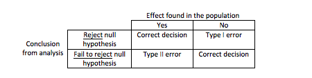
Have this table in mind when designing, analysing and reading studies, it will help when interpreting findings.

Lesson 8: Significance levels and powers of the tests

Course:

Determine the rejection and non-rejection regions
In this step we calculate the significance level . The significance level, also denoted as alpha or α, is the probability of rejecting the null hypothesis when it is true. For example, a significance level of 0.05 indicates a 5% risk of concluding that a difference exists when there is no actual difference.

Determine the value of the test statistics
The values of the test statistic separate the rejection and non-rejection regions.
Rejection region: the set of values for the test statistic that leads to rejection of H₀.
Non-rejection region: the set of values not in the rejection region that leads to non-rejection of H₀.

Lesson 9: p-values

Course:

The P-Value: Another quantitative measure for reporting the result of a test of hypothesis is the p-value. It is also called the probability of chance in order to test. The lower the p-value the greater likelihood of obtaining the same result. And as a result, a low p-value is a good indication that the results are not due to random chance alone. P-value = the probability of obtaining a test statistic equal to or more extreme value than the observed value of H₀. As a result H₀ will be true.
We then compare the p-value with α:
1. If p-value < α, reject H₀.
2. If p-value >= α, do not reject H₀.
3. “If p-value is low, then H₀ must go.”

Lesson 10: Tests for the expected value and variance of random variables

Course:

Select the distribution to use
You can select a sample or the entire population. In selecting the distribution, we must know the mean for the population or the sample.

Population meanIf you know the standard deviation for a population, then you can calculate a confidence interval (CI) for the mean, or average, of that population.  You estimate the population mean,  μ by using a sample mean,   plus or minus a margin of error. The result is called a confidence interval for the population mean, 

Confidence Intervals for Unknown Mean and Known Standard DeviationFor a population with unknown mean μ and known standard deviation α, a confidence interval for the population mean, based on a simple random sample of size n, is   + z^*, where z^* is the upper (1-C)/2 critical value for the standard normal distribution.

To calculate the standard deviation stands for σ is replaced by the estimated standard deviation s, also known as the standard error. Since the standard error is an estimate for the true value of the standard deviation, the distribution of the sample mean  is no longer normal with mean μ and standard deviation . Instead, the sample mean follows the t distribution with mean μ and standard deviation . The t distribution is also described by its degrees of freedom.

Make a decision
Based on the result, you can determine if your study accepts or rejects the null hypothesis.

Lesson 11: Relationship between confidence intervals and hypothesis testing

Course:

If exact p-value is reported, then the relationship between confidence intervals and hypothesis testing is very close.  However, the objective of the two methods is different:

• Hypothesis testing relates to a single conclusion of statistical significance vs. no statistical significance. 
• Confidence intervals provide a range of plausible values for your population.

Which one?

• Use hypothesis testing when you want to do a strict comparison with a pre-specified hypothesis and significance level.
• Use confidence intervals to describe the magnitude of an effect (e.g., mean difference, odds ratio, etc.) or when you want to describe a single sample.

Lesson 12: Practical versus statistical significance

Course:

Practical significance refers to the importance or usefulness of the result in some real-world context. Many sex differences are statistically significant—and may even be interesting for purely scientific reasons—but they are not practically significant. In clinical practice, this same concept is often referred to as “clinical significance.” For example, a study on a new treatment for social phobia might show that it produces a statistically significant positive effect. Yet this effect still might not be strong enough to justify the time, effort, and other costs of putting it into practice—especially if easier and cheaper treatments that work almost as well already exist. Although statistically significant, this result would be said to lack practical or clinical significance.

• Null hypothesis testing is a formal approach to deciding whether a statistical relationship in a sample reflects a real relationship in the population or is just due to chance.
• The logic of null hypothesis testing involves assuming that the null hypothesis is true, finding how likely the sample result would be if this assumption were correct, and then making a decision. If the sample result would be unlikely if the null hypothesis were true, then it is rejected in favor of the alternative hypothesis. If it would not be unlikely, then the null hypothesis is retained.
• The probability of obtaining the sample result if the null hypothesis were true (the p value) is based on two considerations: relationship strength and sample size. Reasonable judgments about whether a sample relationship is statistically significant can often be made by quickly considering these two factors.
• Statistical significance is not the same as relationship strength or importance. Even weak relationships can be statistically significant if the sample size is large enough. It is important to consider relationship strength and the practical significance of a result in addition to its statistical significance.

Assignments:

1. Summarize and provide examples on the measures of central tendency and variability