Hi! Great day! Welcome to this course. Thank you for taking an interest in this course. Learning from this course will help you become adept at it.
What is an Algorithm?
An algorithm is a set of well-defined instructions in sequence to solve a problem.
Qualities of Good Algorithms
- Input and output should be defined precisely.
- Each step in the algorithm should be clear and unambiguous.
- Algorithms should be most effective among many different ways to solve a problem.
- An algorithm shouldn’t include computer code. Instead, the algorithm should be written in such a way that it can be used in different programming languages.
Algorithm Examples
Algorithm to add two numbers
Algorithm to find the largest among three numbers
Algorithm to find all the roots of the quadratic equation
Algorithm to find the factorial
Algorithm to check prime number
Algorithm of Fibonacci series
Algorithm 1: Add two numbers entered by the user
Step 1: Start
Step 2: Declare variables num1, num2 and sum.
Step 3: Read values num1 and num2.
Step 4: Add num1 and num2 and assign the result to sum.
        sum←num1+num2
Step 5: Display sum
Step 6: Stop
Algorithm 2: Find the largest number among three numbers
Step 1: Start
Step 2: Declare variables a,b and c.
Step 3: Read variables a,b and c.
Step 4: If a > b
           If a > c
              Display a is the largest number.
           Else
              Display c is the largest number.
        Else
           If b > c
              Display b is the largest number.
           Else
              Display c is the greatest number.
Step 5: Stop
Algorithm 3: Find Root of the quadratic equatin ax2 + bx + c = 0
Step 1: Start
Step 2: Declare variables a, b, c, D, x1, x2, rp and ip;
Step 3: Calculate discriminant
         D ← b2-4ac
Step 4: If D ≥ 0
              r1 ← (-b+√D)/2a
              r2 ← (-b-√D)/2a
              Display r1 and r2 as roots.
        Else
              Calculate real part and imaginary part
              rp ← -b/2a
              ip ← √(-D)/2a
              Display rp+j(ip) and rp-j(ip) as roots
Step 5: Stop
Algorithm 4: Find the factorial of a number
Step 1: Start
Step 2: Declare variables n, factorial and i.
Step 3: Initialize variables
          factorial ← 1
          i ← 1
Step 4: Read value of n
Step 5: Repeat the steps until i = n
     5.1: factorial ← factorial*i
     5.2: i ← i+1
Step 6: Display factorial
Step 7: Stop
Algorithm 5: Check whether a number is prime or not
Step 1: Start
Step 2: Declare variables n, i, flag.
Step 3: Initialize variables
        flag ← 1
        i ← 2
Step 4: Read n from the user.
Step 5: Repeat the steps until i=(n/2)
     5.1 If remainder of n÷i equals 0
            flag ← 0
            Go to step 6
     5.2 i ← i+1
Step 6: If flag = 0
           Display n is not prime
        else
           Display n is prime
Step 7: Stop
Algorithm 6: Find the Fibonacci series till the term less than 1000
Step 1: Start
Step 2: Declare variables first_term,second_term and temp.
Step 3: Initialize variables first_term ← 0 second_term ← 1
Step 4: Display first_term and second_term
Step 5: Repeat the steps until second_term ≤ 1000
     5.1: temp ← second_term
     5.2: second_term ← second_term + first_term
     5.3: first_term ← temp
     5.4: Display second_term
Step 6: Stop
Why Learn Data Structures and Algorithms?
What are Algorithms?
Informally, an algorithm is nothing but a mention of steps to solve a problem. They are essentially a solution.
For example, an algorithm to solve the problem of factorials might look something like this:
Problem: Find the factorial of n
Initialize fact = 1
For every value v in range 1 to n:
    Multiply the fact by v
fact contains the factorial of n
Here, the algorithm is written in English. If it was written in a programming language, we would call it to code instead. Here is a code for finding the factorial of a number in C++.
int factorial(int n) {
    int fact = 1;
    for (int v = 1; v <= n; v++) {
        fact = fact * v;
    }
    return fact;
}
Programming is all about data structures and algorithms. Data structures are used to hold data while algorithms are used to solve the problem using that data.
Data structures and algorithms (DSA) goes through solutions to standard problems in detail and gives you an insight into how efficient it is to use each one of them. It also teaches you the science of evaluating the efficiency of an algorithm. This enables you to choose the best of various choices.
Use of Data Structures and Algorithms to Make Your Code Scalable
Time is precious.
Suppose, Alice and Bob are trying to solve a simple problem of finding the sum of the first 1011 natural numbers. While Bob was writing the algorithm, Alice implemented it proving that it is as simple as criticizing Donald Trump.
Algorithm (by Bob)
Initialize sum = 0
for every natural number n in range 1 to 1011 (inclusive):
    add n to sum
sum is your answer
Code (by Alice)
int findSum() {
    int sum = 0;
    for (int v = 1; v <= 100000000000; v++) {
        sum += v;
    }
    return sum;
}
Alice and Bob are feeling euphoric of themselves that they could build something of their own in almost no time. Let’s sneak into their workspace and listen to their conversation.
Alice: Let's run this code and find out the sum.
Bob: I ran this code a few minutes back but it's still not showing the output. What's wrong with it?
Oops, something went wrong! A computer is the most deterministic machine. Going back and trying to run it again won’t help. So let’s analyze what’s wrong with this simple code.
Two of the most valuable resources for a computer program are time and memory.
The time taken by the computer to run code is:
Time to run code = number of instructions * time to execute each instruction
The number of instructions depends on the code you used, and the time taken to execute each code depends on your machine and compiler.
In this case, the total number of instructions executed (let’s say x) are x = 1 + (1011 + 1) + (1011) + 1, which is x = 2 * 1011 + 3
Let us assume that a computer can execute y = 108 instructions in one second (it can vary subject to machine configuration). The time taken to run above code is
Time taken to run code = x/y (greater than 16 minutes)
Is it possible to optimize the algorithm so that Alice and Bob do not have to wait for 16 minutes every time they run this code?
I am sure that you already guessed the right method. The sum of first N natural numbers is given by the formula:
Sum = N * (N + 1) / 2
Converting it into code will look something like this:
int sum(int N) {
    return N * (N + 1) / 2;
}
This code executes in just one instruction and gets the task done no matter what the value is. Let it be greater than the total number of atoms in the universe. It will find the result in no time.
The time taken to solve the problem, in this case, is 1/y (which is 10 nanoseconds). By the way, the fusion reaction of a hydrogen bomb takes 40-50 ns, which means your program will complete successfully even if someone throws a hydrogen bomb on your computer at the same time you ran your code. 🙂
Note: Computers take a few instructions (not 1) to compute multiplication and division. I have said 1 just for the sake of simplicity.
More on Scalability
Scalability is scale plus ability, which means the quality of an algorithm/system to handle the problem of larger size.
Consider the problem of setting up a classroom of 50 students. One of the simplest solutions is to book a room, get a blackboard, a few chalks, and the problem is solved.
But what if the size of the problem increases? What if the number of students increased to 200?
The solution still holds but it needs more resources. In this case, you will probably need a much larger room (probably a theater), a projector screen and a digital pen.
What if the number of students increased to 1000?
The solution fails or uses a lot of resources when the size of the problem increases. This means, your solution wasn’t scalable.
What is a scalable solution then?
Consider a site like Khanacademy, millions of students can see videos, read answers at the same time and no more resources are required. So, the solution can solve the problems of larger size under resource crunch.
If you see our first solution to find the sum of first N natural numbers, it wasn’t scalable. It’s because it required linear growth in time with the linear growth in the size of the problem. Such algorithms are also known as linearly scalable algorithms.
Our second solution was very scalable and didn’t require the use of any more time to solve a problem of larger size. These are known as constant-time algorithms.
Memory is expensive
Memory is not always available in abundance. While dealing with code/system which requires you to store or produce a lot of data, it is critical for your algorithm to save the usage of memory wherever possible. For example: While storing data about people, you can save memory by storing only their age not the date of birth. You can always calculate it on the fly using their age and current date.
Examples of an Algorithm’s Efficiency
Here are some examples of what learning algorithms and data structures enable you to do:
Example 1: Age Group Problem
Problems like finding the people of a certain age group can easily be solved with a little modified version of the binary search algorithm (assuming that the data is sorted).
The naive algorithm which goes through all the persons one by one, and checks if it falls in the given age group is linearly scalable. Whereas, binary search claims itself to be a logarithmically scalable algorithm. This means that if the size of the problem is squared, the time taken to solve it is only doubled.
Suppose, it takes 1 second to find all the people at a certain age for a group of 1000. Then for a group of 1 million people,
- the binary search algorithm will take only 2 seconds to solve the problem
- the naive algorithm might take 1 million seconds, which is around 12 days
The same binary search algorithm is used to find the square root of a number.
Example 2: Rubik’s Cube Problem
Imagine you are writing a program to find the solution of a Rubik’s cube.
This cute looking puzzle has annoyingly 43,252,003,274,489,856,000 positions, and these are just positions! Imagine the number of paths one can take to reach the wrong positions.
Fortunately, the way to solve this problem can be represented by the graph data structure. There is a graph algorithm known as Dijkstra’s algorithm which allows you to solve this problem in linear time. Yes, you heard it right. It means that it allows you to reach the solved position in a minimum number of states.
Example 3: DNA Problem
DNA is a molecule that carries genetic information. They are made up of smaller units which are represented by Roman characters A, C, T, and G.
Imagine yourself working in the field of bioinformatics. You are assigned the work of finding out the occurrence of a particular pattern in a DNA strand.
It is a famous problem in computer science academia. And, the simplest algorithm takes the time proportional to
(number of character in DNA strand) * (number of characters in pattern)
A typical DNA strand has millions of such units. Eh! worry not. KMP algorithm can get this done in time which is proportional to
(number of character in DNA strand) + (number of characters in pattern)
The * operator replaced by + makes a lot of change.
Considering that the pattern was of 100 characters, your algorithm is now 100 times faster. If your pattern was of 1000 characters, the KMP algorithm would be almost 1000 times faster. That is, if you were able to find the occurrence of pattern in 1 second, it will now take you just 1 ms. We can also put this in another way. Instead of matching 1 strand, you can match 1000 strands of similar length at the same time.
And there are infinite such stories…
Final Words
Generally, software development involves learning new technologies on a daily basis. You get to learn most of these technologies while using them in one of your projects. However, it is not the case with algorithms.
If you don’t know algorithms well, you won’t be able to identify if you can optimize the code you are writing right now. You are expected to know them in advance and apply them wherever possible and critical.
We specifically talked about the scalability of algorithms. A software system consists of many such algorithms. Optimizing any one of them leads to a better system.
However, it’s important to note that this is not the only way to make a system scalable. For example, a technique known as distributed computing allows independent parts of a program to run to multiple machines together making it even more scalable.
Divide and Conquer Algorithm
A divide and conquer algorithm is a strategy of solving a large problem by
- breaking the problem into smaller sub-problems
- solving the sub-problems, and
- combining them to get the desired output.
To use the divide and conquer algorithm, recursion is used. Learn about recursion in different programming languages:
- Recursion in Java
- Recursion in Python
- Recursion in C++
How Divide and Conquer Algorithms Work?
Here are the steps involved:
- Divide: Divide the given problem into sub-problems using recursion.
- Conquer: Solve the smaller sub-problems recursively. If the subproblem is small enough, then solve it directly.
- Combine: Combine the solutions of the sub-problems that are part of the recursive process to solve the actual problem.
Let us understand this concept with the help of an example.
Here, we will sort an array using the divide and conquer approach (ie. merge sort).
- Let the given array be:
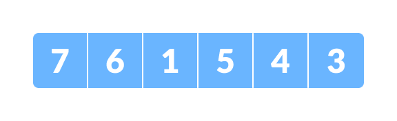 Array for merge sort
 - Divide the array into two halves.
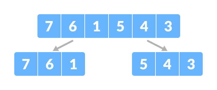 Divide the array into two subparts
Again, divide each subpart recursively into two halves until you get individual elements.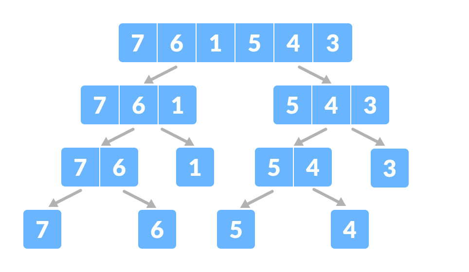 Divide the array into smaller subparts
 - Now, combine the individual elements in a sorted manner. Here, conquer and combine steps go side by side.
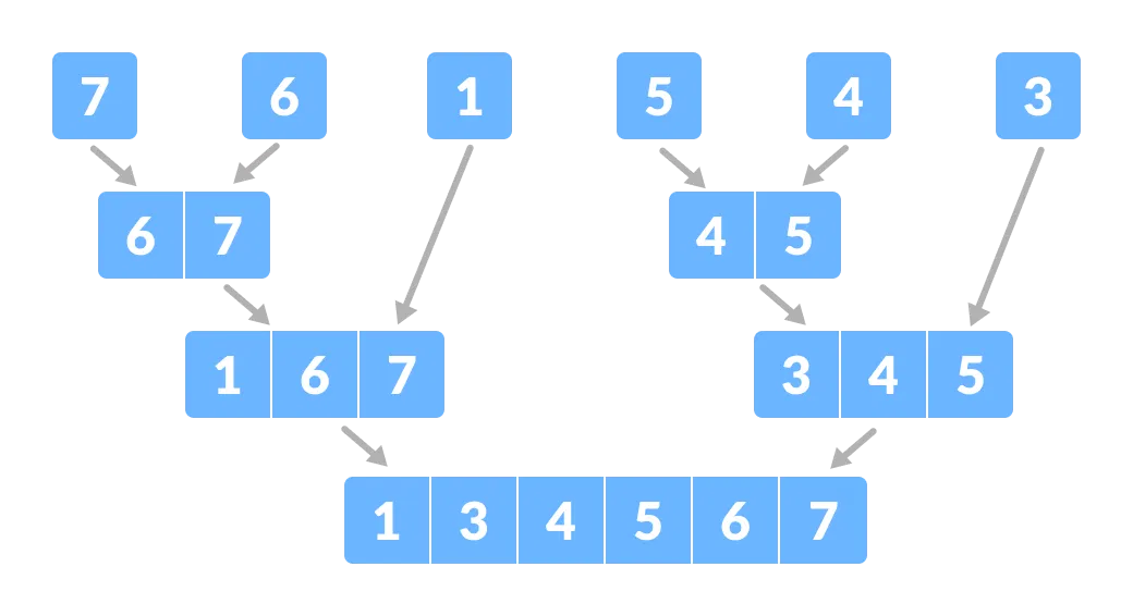 Combine the subparts
Time Complexity
The complexity of the divide and conquer algorithm is calculated using the master theorem.
T(n) = aT(n/b) + f(n),
where,
n = size of input
a = number of subproblems in the recursion
n/b = size of each subproblem. All subproblems are assumed to have the same size.
f(n) = cost of the work done outside the recursive call, which includes the cost of dividing the problem and cost of merging the solutions
Let us take an example to find the time complexity of a recursive problem.
For a merge sort, the equation can be written as:
T(n) = aT(n/b) + f(n)
     = 2T(n/2) + O(n)
Where,
a = 2 (each time, a problem is divided into 2 subproblems)
n/b = n/2 (size of each sub problem is half of the input)
f(n) = time taken to divide the problem and merging the subproblems
T(n/2) = O(n log n) (To understand this, please refer to the master theorem.)

Now, T(n) = 2T(n log n) + O(n)
          ≈ O(n log n)
Divide and Conquer Vs Dynamic approach
The divide and conquer approach divides a problem into smaller subproblems; these subproblems are further solved recursively. The result of each subproblem is not stored for future reference, whereas, in a dynamic approach, the result of each subproblem is stored for future reference.
Use the divide and conquer approach when the same subproblem is not solved multiple times. Use the dynamic approach when the result of a subproblem is to be used multiple times in the future.
Let us understand this with an example. Suppose we are trying to find the Fibonacci series. Then,
Divide and Conquer approach:
fib(n)
    If n < 2, return 1
    Else , return f(n - 1) + f(n -2)
Dynamic approach:
mem = []
fib(n)
    If n in mem: return mem[n]
    else,
        If n < 2, f = 1
        else , f = f(n - 1) + f(n -2)
        mem[n] = f
        return f
In a dynamic approach, mem stores the result of each subproblem.
Advantages of Divide and Conquer Algorithm
- The complexity for the multiplication of two matrices using the naive method is O(n3), whereas using the divide and conquer approach (i.e. Strassen’s matrix multiplication) is O(n2.8074). This approach also simplifies other problems, such as the Tower of Hanoi.
- This approach is suitable for multiprocessing systems.
- It makes efficient use of memory caches.
Divide and Conquer Applications
- Binary Search
- Merge Sort
- Quick Sort
- Strassen’s Matrix multiplication
- Karatsuba Algorithm
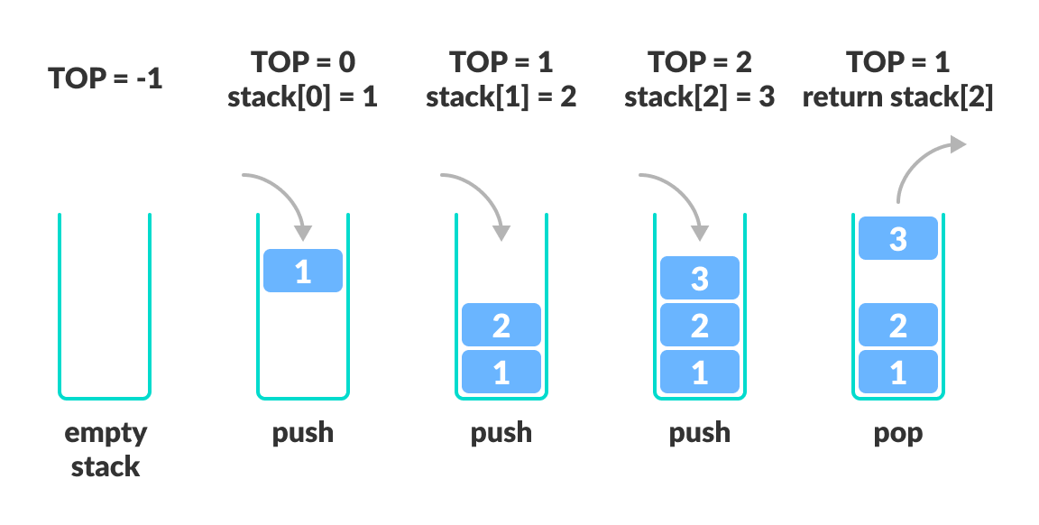
Stack Data Structure
A stack is a useful data structure in programming. It is just like a pile of plates kept on top of each other.

Think about the things you can do with such a pile of plates
- Put a new plate on top
- Remove the top plate
If you want the plate at the bottom, you must first remove all the plates on top. Such an arrangement is called Last In First Out – the last item that is the first item to go out.
LIFO Principle of Stack
In programming terms, putting an item on top of the stack is called push and removing an item is called pop.

In the above image, although item 2 was kept last, it was removed first – so it follows the Last In First Out(LIFO) principle.
We can implement a stack in any programming language like C, C++, Java, Python or C#, but the specification is pretty much the same.
Basic Operations of Stack
A stack is an object (an abstract data type – ADT) that allows the following operations:
- Push: Add an element to the top of a stack
- Pop: Remove an element from the top of a stack
- IsEmpty: Check if the stack is empty
- IsFull: Check if the stack is full
- Peek: Get the value of the top element without removing it
Working of Stack Data Structure
The operations work as follows:
- A pointer called TOP is used to keep track of the top element in the stack.
- When initializing the stack, we set its value to -1 so that we can check if the stack is empty by comparing
TOP == -1. - On pushing an element, we increase the value of TOP and place the new element in the position pointed to by TOP.
- On popping an element, we return the element pointed to by TOP and reduce its value.
- Before pushing, we check if the stack is already full
- Before popping, we check if the stack is already empty
Stack Implementations in Python, Java, C, and C++
The most common stack implementation is using arrays, but it can also be implemented using lists.PythonJavaCC+
# Stack implementation in python


# Creating a stack
def create_stack():
    stack = []
    return stack


# Creating an empty stack
def check_empty(stack):
    return len(stack) == 0


# Adding items into the stack
def push(stack, item):
    stack.append(item)
    print("pushed item: " + item)


# Removing an element from the stack
def pop(stack):
    if (check_empty(stack)):
        return "stack is empty"

    return stack.pop()


stack = create_stack()
push(stack, str(1))
push(stack, str(2))
push(stack, str(3))
push(stack, str(4))
print("popped item: " + pop(stack))
print("stack after popping an element: " + str(stack))
Stack Time Complexity
For the array-based implementation of a stack, the push and pop operations take constant time, i.e. O(1).
Applications of Stack Data Structure
Although stack is a simple data structure to implement, it is very powerful. The most common uses of a stack are:
- To reverse a word – Put all the letters in a stack and pop them out. Because of the LIFO order of stack, you will get the letters in reverse order.
- In compilers – Compilers use the stack to calculate the value of expressions like
2 + 4 / 5 * (7 - 9)by converting the expression to prefix or postfix form. - In browsers – The back button in a browser saves all the URLs you have visited previously in a stack. Each time you visit a new page, it is added on top of the stack. When you press the back button, the current URL is removed from the stack, and the previous URL is accessed.
Queue Data Structure
A queue is a useful data structure in programming. It is similar to the ticket queue outside a cinema hall, where the first person entering the queue is the first person who gets the ticket.
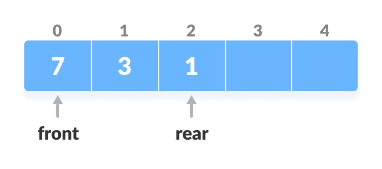
Queue follows the First In First Out (FIFO) rule – the item that goes in first is the item that comes out first.

In the above image, since 1 was kept in the queue before 2, it is the first to be removed from the queue as well. It follows the FIFO rule.
In programming terms, putting items in the queue is called enqueue, and removing items from the queue is called dequeue.
We can implement the queue in any programming language like C, C++, Java, Python or C#, but the specification is pretty much the same.
Basic Operations of Queue
A queue is an object (an abstract data structure – ADT) that allows the following operations:
- Enqueue: Add an element to the end of the queue
- Dequeue: Remove an element from the front of the queue
- IsEmpty: Check if the queue is empty
- IsFull: Check if the queue is full
- Peek: Get the value of the front of the queue without removing it
Working of Queue
Queue operations work as follows:
- two pointers FRONT and REAR
- FRONT track the first element of the queue
- REAR track the last element of the queue
- initially, set value of FRONT and REAR to -1
Enqueue Operation
- check if the queue is full
- for the first element, set the value of FRONT to 0
- increase the REAR index by 1
- add the new element in the position pointed to by REAR
Dequeue Operation
- check if the queue is empty
- return the value pointed by FRONT
- increase the FRONT index by 1
- for the last element, reset the values of FRONT and REAR to -1

Queue Implementations in Python, Java, C, and C++
We usually use arrays to implement queues in Java and C/++. In the case of Python, we use lists.PythonJavaCC++
# Queue implementation in Python

class Queue:

    def __init__(self):
        self.queue = []

    # Add an element
    def enqueue(self, item):
        self.queue.append(item)

    # Remove an element
    def dequeue(self):
        if len(self.queue) < 1:
            return None
        return self.queue.pop(0)

    # Display  the queue
    def display(self):
        print(self.queue)

    def size(self):
        return len(self.queue)


q = Queue()
q.enqueue(1)
q.enqueue(2)
q.enqueue(3)
q.enqueue(4)
q.enqueue(5)

q.display()

q.dequeue()

print("After removing an element")
q.display()
Limitations of Queue
As you can see in the image below, after a bit of enqueuing and dequeuing, the size of the queue has been reduced.

And we can only add indexes 0 and 1 only when the queue is reset (when all the elements have been dequeued).
After REAR reaches the last index, if we can store extra elements in the empty spaces (0 and 1), we can make use of the empty spaces. This is implemented by a modified queue called the circular queue.
Complexity Analysis
The complexity of enqueue and dequeue operations in a queue using an array is O(1).
Applications of Queue
- CPU scheduling, Disk Scheduling
- When data is transferred asynchronously between two processes.The queue is used for synchronization. For example: IO Buffers, pipes, file IO, etc
- Handling of interrupts in real-time systems.
- Call Center phone systems use Queues to hold people calling them in order.
Recommended Readings
- Types of Queue
- Circular Queue
- Deque Data Structure
- Priority Queue
Types of Queues
A queue is a useful data structure in programming. It is similar to the ticket queue outside a cinema hall, where the first person entering the queue is the first person who gets the ticket.
There are four different types of queues:
- Simple Queue
- Circular Queue
- Priority Queue
- Double Ended Queue
Simple Queue
In a simple queue, insertion takes place at the rear and removal occurs at the front. It strictly follows the FIFO (First in First out) rule.

To learn more, visit Queue Data Structure.
Circular Queue
In a circular queue, the last element points to the first element making a circular link.

The main advantage of a circular queue over a simple queue is better memory utilization. If the last position is full and the first position is empty, we can insert an element in the first position. This action is not possible in a simple queue.
To learn more, visit Circular Queue Data Structure.
Priority Queue
A priority queue is a special type of queue in which each element is associated with a priority and is served according to its priority. If elements with the same priority occur, they are served according to their order in the queue.

Insertion occurs based on the arrival of the values and removal occurs based on priority.
To learn more, visit Priority Queue Data Structure.
Deque (Double Ended Queue)
In a double ended queue, insertion and removal of elements can be performed from either from the front or rear. Thus, it does not follow the FIFO (First In First Out) rule.

To learn more, visit Deque Data Structure.
Circular Queue Data Structure
Circular queue avoids the wastage of space in a regular queue implementation using arrays.

As you can see in the above image, after a bit of enqueuing and dequeuing, the size of the queue has been reduced.
The indexes 0 and 1 can only be used after the queue is reset when all the elements have been dequeued.
How Circular Queue Works
Circular Queue works by the process of circular increment i.e. when we try to increment the pointer and we reach the end of the queue, we start from the beginning of the queue.
Here, the circular increment is performed by modulo division with the queue size. That is,
if REAR + 1 == 5 (overflow!), REAR = (REAR + 1)%5 = 0 (start of queue)

Circular Queue Operations
The circular queue work as follows:
- two pointers FRONT and REAR
- FRONT track the first element of the queue
- REAR track the last elements of the queue
- initially, set value of FRONT and REAR to -1
1. Enqueue Operation
- check if the queue is full
- for the first element, set value of FRONT to 0
- circularly increase the REAR index by 1 (i.e. if the rear reaches the end, next it would be at the start of the queue)
- add the new element in the position pointed to by REAR
2. Dequeue Operation
- check if the queue is empty
- return the value pointed by FRONT
- circularly increase the FRONT index by 1
- for the last element, reset the values of FRONT and REAR to -1
However, the check for full queue has a new additional case:
- Case 1: FRONT = 0 &&
REAR == SIZE - 1 - Case 2:
FRONT = REAR + 1
The second case happens when REAR starts from 0 due to circular increment and when its value is just 1 less than FRONT, the queue is full.

Circular Queue Implementations in Python, Java, C, and C++
The most common queue implementation is using arrays, but it can also be implemented using lists.PythonJavaCC+
# Circular Queue implementation in Python


class MyCircularQueue():

    def __init__(self, k):
        self.k = k
        self.queue = [None] * k
        self.head = self.tail = -1

    # Insert an element into the circular queue
    def enqueue(self, data):

        if ((self.tail + 1) % self.k == self.head):
            print("The circular queue is full\n")

        elif (self.head == -1):
            self.head = 0
            self.tail = 0
            self.queue[self.tail] = data
        else:
            self.tail = (self.tail + 1) % self.k
            self.queue[self.tail] = data

    # Delete an element from the circular queue
    def dequeue(self):
        if (self.head == -1):
            print("The circular queue is empty\n")

        elif (self.head == self.tail):
            temp = self.queue[self.head]
            self.head = -1
            self.tail = -1
            return temp
        else:
            temp = self.queue[self.head]
            self.head = (self.head + 1) % self.k
            return temp

    def printCQueue(self):
        if(self.head == -1):
            print("No element in the circular queue")

        elif (self.tail >= self.head):
            for i in range(self.head, self.tail + 1):
                print(self.queue[i], end=" ")
            print()
        else:
            for i in range(self.head, self.k):
                print(self.queue[i], end=" ")
            for i in range(0, self.tail + 1):
                print(self.queue[i], end=" ")
            print()


# Your MyCircularQueue object will be instantiated and called as such:
obj = MyCircularQueue(5)
obj.enqueue(1)
obj.enqueue(2)
obj.enqueue(3)
obj.enqueue(4)
obj.enqueue(5)
print("Initial queue")
obj.printCQueue()

obj.dequeue()
print("After removing an element from the queue")
obj.printCQueue()
Circular Queue Complexity Analysis
The complexity of the enqueue and dequeue operations of a circular queue is O(1) for (array implementations).
Priority Queue
A priority queue is a special type of queue in which each element is associated with a priority and is served according to its priority. If elements with the same priority occur, they are served according to their order in the queue.
Generally, the value of the element itself is considered for assigning the priority.
For example, The element with the highest value is considered as the highest priority element. However, in other cases, we can assume the element with the lowest value as the highest priority element. In other cases, we can set priorities according to our needs.

Difference between Priority Queue and Normal Queue
In a queue, the first-in-first-out rule is implemented whereas, in a priority queue, the values are removed on the basis of priority. The element with the highest priority is removed first.
Implementation of Priority Queue
Priority queue can be implemented using an array, a linked list, a heap data structure, or a binary search tree. Among these data structures, heap data structure provides an efficient implementation of priority queues.
Hence, we will be using the heap data structure to implement the priority queue in this tutorial. A max-heap is implement is in the following operations. If you want to learn more about it, please visit max-heap and mean-heap.
A comparative analysis of different implementations of priority queue is given below.
| Operations | peek | insert | delete |
|---|---|---|---|
| Linked List | O(1) | O(n) | O(1) |
| Binary Heap | O(1) | O(log n) | O(log n) |
| Binary Search Tree | O(1) | O(log n) | O(log n) |
Priority Queue Operations
Basic operations of a priority queue are inserting, removing, and peeking elements.
Before studying the priority queue, please refer to the heap data structure for a better understanding of binary heap as it is used to implement the priority queue in this article.
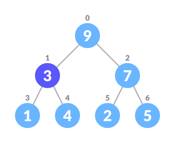
1. Inserting an Element into the Priority Queue
Inserting an element into a priority queue (max-heap) is done by the following steps.
- Insert the new element at the end of the tree.
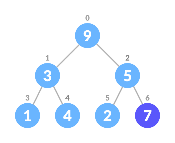 Insert an element at the end of the queue
 - Heapify the tree.
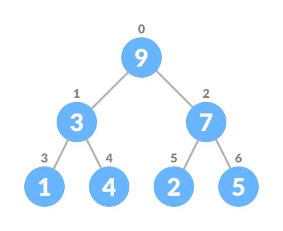 Heapify after insertion
Algorithm for insertion of an element into priority queue (max-heap)
If there is no node,
  create a newNode.
else (a node is already present)
  insert the newNode at the end (last node from left to right.)

heapify the array
For Min Heap, the above algorithm is modified so that parentNode is always smaller than newNode.
2. Deleting an Element from the Priority Queue
Deleting an element from a priority queue (max-heap) is done as follows:
- Select the element to be deleted.
 Select the element to be deleted
 - Swap it with the last element.
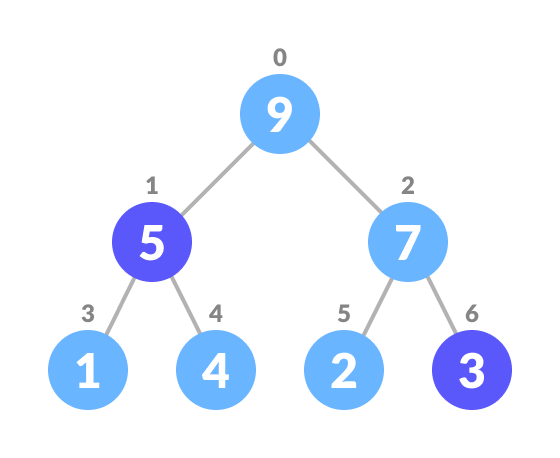 Swap with the last leaf node element
 - Remove the last element.
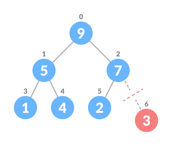 Remove the last element leaf
 - Heapify the tree.
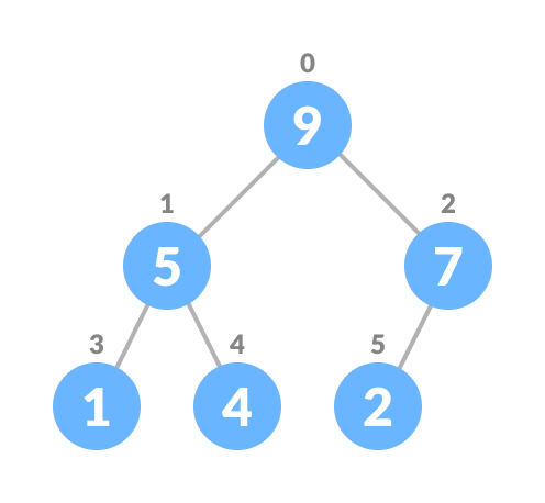 Heapify the priority queue
Algorithm for deletion of an element in the priority queue (max-heap)
If nodeToBeDeleted is the leafNode
  remove the node
Else swap nodeToBeDeleted with the lastLeafNode
  remove noteToBeDeleted

heapify the array
For Min Heap, the above algorithm is modified so that the both childNodes are smaller than currentNode.
3. Peeking from the Priority Queue (Find max/min)
Peek operation returns the maximum element from Max Heap or minimum element from Min Heap without deleting the node.
For both Max heap and Min Heap
return rootNode
4. Extract-Max/Min from the Priority Queue
Extract-Max returns the node with maximum value after removing it from a Max Heap whereas Extract-Min returns the node with minimum value after removing it from Min Heap.
Priority Queue Implementations in Python, Java, C, and C++
PythonJavaCC++
# Priority Queue implementation in Python


# Function to heapify the tree
def heapify(arr, n, i):
    # Find the largest among root, left child and right child
    largest = i
    l = 2 * i + 1
    r = 2 * i + 2

    if l < n and arr[i] < arr[l]:
        largest = l

    if r < n and arr[largest] < arr[r]:
        largest = r

    # Swap and continue heapifying if root is not largest
    if largest != i:
        arr[i], arr[largest] = arr[largest], arr[i]
        heapify(arr, n, largest)


# Function to insert an element into the tree
def insert(array, newNum):
    size = len(array)
    if size == 0:
        array.append(newNum)
    else:
        array.append(newNum)
        for i in range((size // 2) - 1, -1, -1):
            heapify(array, size, i)


# Function to delete an element from the tree
def deleteNode(array, num):
    size = len(array)
    i = 0
    for i in range(0, size):
        if num == array[i]:
            break

    array[i], array[size - 1] = array[size - 1], array[i]

    array.remove(size - 1)

    for i in range((len(array) // 2) - 1, -1, -1):
        heapify(array, len(array), i)


arr = []

insert(arr, 3)
insert(arr, 4)
insert(arr, 9)
insert(arr, 5)
insert(arr, 2)

print ("Max-Heap array: " + str(arr))

deleteNode(arr, 4)
print("After deleting an element: " + str(arr))
Deque Data Structure
Deque or Double Ended Queue is a type of queue in which insertion and removal of elements can be performed from either from the front or rear. Thus, it does not follow FIFO rule (First In First Out).

Types of Deque
- Input Restricted Deque
In this deque, input is restricted at a single end but allows deletion at both the ends. - Output Restricted Deque
In this deque, output is restricted at a single end but allows insertion at both the ends.
Operations on a Deque
Below is the circular array implementation of deque. In a circular array, if the array is full, we start from the beginning.
But in a linear array implementation, if the array is full, no more elements can be inserted. In each of the operations below, if the array is full, “overflow message” is thrown.
Before performing the following operations, these steps are followed.
- Take an array (deque) of size n.
- Set two pointers at the first position and set
front = -1andrear = 0.

1. Insert at the Front
This operation adds an element at the front.
- Check the position of front.
 Check the position of front
 - If
front < 1, reinitializefront = n-1(last index).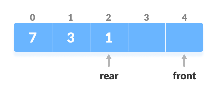 Shift front to the end
 - Else, decrease front by 1.
- Add the new key 5 into
array[front].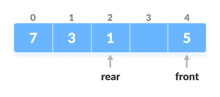 Insert the element at Front
2. Insert at the Rear
This operation adds an element to the rear.
- Check if the array is full.
 Check if deque is full
 - If the deque is full, reinitialize
rear = 0. - Else, increase rear by 1.
 Increase the rear
 - Add the new key 5 into
array[rear]. Insert the element at rear
3. Delete from the Front
The operation deletes an element from the front.
- Check if the deque is empty.
 Check if deque is empty
 - If the deque is empty (i.e.
front = -1), deletion cannot be performed (underflow condition). - If the deque has only one element (i.e.
front = rear), setfront = -1andrear = -1. - Else if front is at the end (i.e.
front = n - 1), set go to the frontfront = 0. - Else,
front = front + 1.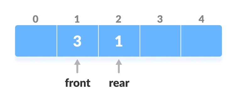 Increase the front
4. Delete from the Rear
This operation deletes an element from the rear.
- Check if the deque is empty.
 Check if deque is empty
 - If the deque is empty (i.e.
front = -1), deletion cannot be performed (underflow condition). - If the deque has only one element (i.e.
front = rear), setfront = -1andrear = -1, else follow the steps below. - If rear is at the front (i.e.
rear = 0), set go to the frontrear = n - 1. - Else,
rear = rear - 1.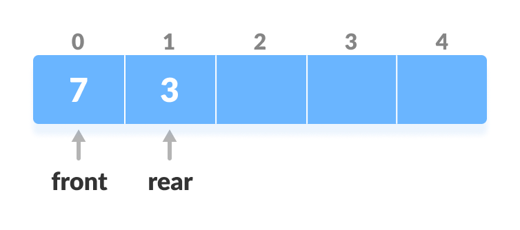 Decrease the rear
5. Check Empty
This operation checks if the deque is empty. If front = -1, the deque is empty.
6. Check Full
This operation checks if the deque is full. If front = 0 and rear = n - 1 OR front = rear + 1, the deque is full.
Deque Implementation in Python, Java, C, and C++
PythonJavaCC++
# Deque implementaion in python

class Deque:
    def __init__(self):
        self.items = []

    def isEmpty(self):
        return self.items == []

    def addRear(self, item):
        self.items.append(item)

    def addFront(self, item):
        self.items.insert(0, item)

    def removeFront(self):
        return self.items.pop()

    def removeRear(self):
        return self.items.pop(0)

    def size(self):
        return len(self.items)


d = Deque()
print(d.isEmpty())
d.addRear(8)
d.addRear(5)
d.addFront(7)
d.addFront(10)
print(d.size())
print(d.isEmpty())
d.addRear(11)
print(d.removeRear())
print(d.removeFront())
d.addFront(55)
d.addRear(45)
print(d.items)
Time Complexity
The time complexity of all the above operations is constant i.e. O(1).
Mini Project:
- Video record in mp4 format while programming the different structures and algorithms
Assignment:
- Discuss all the lessons in your own words and use pictures of your mini project to explain it better in PPT.